Mediative recently hosted a Apache Spark Montreal Meetup’s project night where some of us decided to create a simple ML pipeline.
To spare the installation of Spark, we used the Databricks community edition.
Since the goal was to see if we could make it work,
we wanted to use data that we knew was correlated.
But to make the project a little more fun,
we decided to explore something else than the usual data sets
so we went for the Dow Jones and Nasdaq.
In the wealth of all R packages, one can find the quantmod package to access financial data.
Getting data
The notebook was created for Scala language, so we used the %r magic to install and use the R package to access the data. And while we were at it, we merge both data sets right away:
%r
install.packages("quantmod")
library("quantmod")

## NASDAQ
nsd<-as.data.frame(getSymbols(Symbols = "^NDX",
    src = "yahoo", from = "2015-01-01",to = "2016-01-01", env = NULL))
## Dow Jones
dji<-as.data.frame(getSymbols(Symbols = "^DJI",
    src = "yahoo", from = "2015-01-01",to = "2016-01-01", env = NULL))

## Adding the date as a column (in the above they are index and are lost when a table is created)
nsd$date<-rownames(nsd)
dji$date<-rownames(dji)

## Merge the tables together on date
mrgIndx<-merge(nsd, dji)

dfIndx <- createDataFrame(sqlContext, mrgIndx)
registerTempTable(dfIndx, "testIndx")
The last line register the dataframe as a (temporary) table to make it available outside of the R scope.
The following (default) scala cell will create a dataframe back from this table.
val df = sqlContext.sql("SELECT * FROM testIndx")
Looking at the data
Of all the fields, we will only consider the date and the adjusted Nasdaq,NDX_Adjusted, and Dow Jones, DJI_Adjusted values. Why adjusted? No reason, so why not! Let see if they are correlated and we can have hope to predict one with the other:
import org.apache.spark.sql.functions.lit
display(df.withColumn("NDXTimes5", $"NDX_Adjusted".cast(DoubleType).multiply(lit(5))))
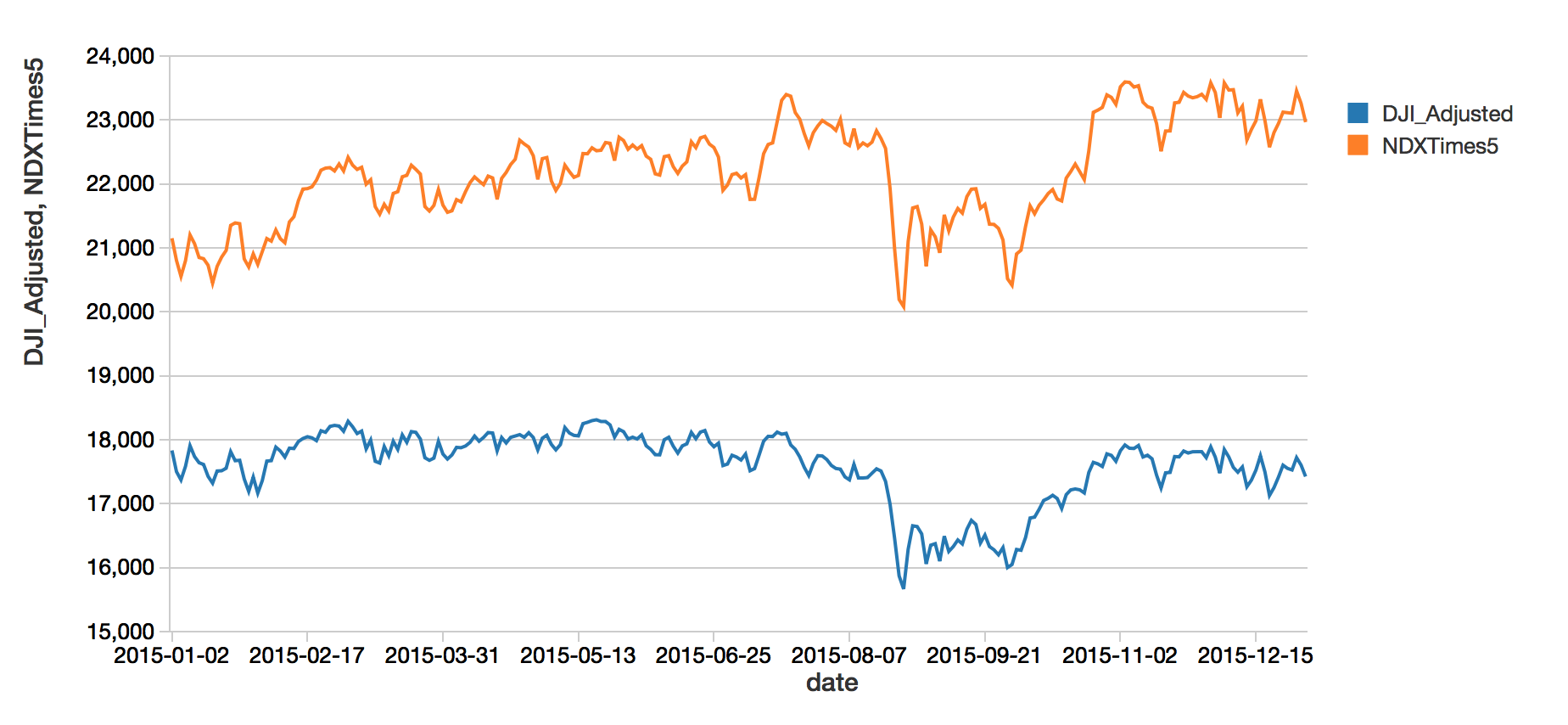
No fancy statistical tools are needed to see that these two curves are correlated. The Nasdaq value has been scaled up by five (using the imported lit function) to make the comparison more obvious, but this scaling will not be used in the training. Hopefully, even a basic model can take care of that.
Preparing the data and the model
Let’s keep only the fields that we will need
val data = df.withColumn("NDX", $"NDX_Adjusted")
.withColumn("DJI", $"DJI_Adjusted")
.select("NDX", "DJI")
And let’s keep a random test subsample for testing purpose, the rest will be use for training the model.
val Array(training, test) = data.randomSplit(Array(0.75, 0.25), seed = 12345)
We use the VectorAssembler to create the feature vector used by the model. We want to predict the Dow Jones with the Nasdaq (NDX), so the latter will be our feature, which we will wisely call features.
import org.apache.spark.ml.feature.VectorAssembler
val assembler = new VectorAssembler()
  .setInputCols(Array("NDX"))
  .setOutputCol("features")
We will also need a model to learn with, for such a simple task, let’s use a simple linear regression where we define the Dow Jones (DJI) as the target we want to learn on (that is called label in ml).
import org.apache.spark.ml.regression.LinearRegression
val lr = new LinearRegression()
  .setLabelCol("DJI")
  .setFeaturesCol("features")
Set up the pipeline
Now that we have all the elements, we can easily assemble them with the pipeline functionality.
import org.apache.spark.ml.Pipeline
val steps: Array[org.apache.spark.ml.PipelineStage] = Array(assembler, lr)
val pipeline = new Pipeline().setStages(steps)
Fitting the model
Preparing data and training is done with a single call of the pipeline
val myModel = pipeline.fit(training)
We can now see how well the model works by comparing its prediction with the actual Dow Jones values
display(myModel.transform(test).select("prediction", "DJI"))
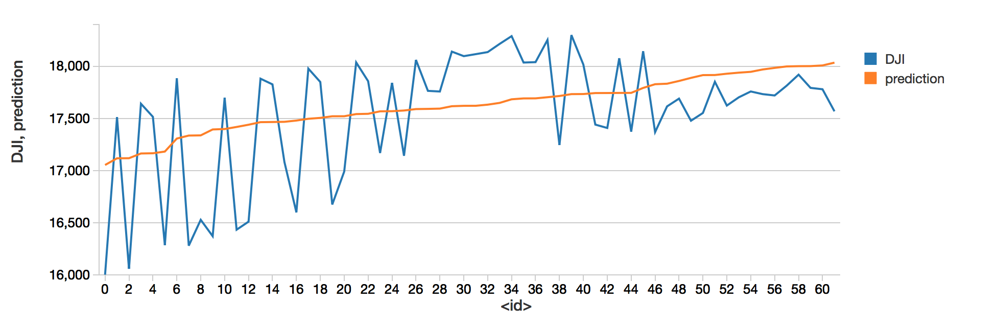
The model obviously managed to learn correlations between the Dow jones and the Nasdaq. Nothing to impress your broker, but that is a basis on which building better prediction.